Circumferential Length
Contents
Circumferential Length#
Circumferential Length#
Definition: Curvature length from a set of points roughtly alinged in a plane perpendicular to the longitudinal axis.
The circumferential length is calculated as the length of a curve inscribed within myocardial region along the circumferential axis. In our solution, we constructed these curves based on given speckles, thus we are essentially determining the “speckle length”. To guarantee that this metric is consistent with its definition, the normal of the plane of reference for these speckles must be parallel to the normal axis.
Here is an example:
[2]:
sample_spk_ideal = lv_ideal.get_speckles(spk_name="SAMPLE", spk_group="epi", spk_collection="SAMPLE")
[3]:
lv_ideal.plot_speckles(sample_spk_ideal[-1],
cmap="tab20",
point_size=200,
add_k_centers=True,
k_centers_as_line=True,
k_bins=True,
t=0.0)
As speckles are pre-defined during initialization, their corresponing mesh ids are fixed, which allows us to ‘draw’ a line between clusters inside a speckle and track their deformation throughout timesteps.
[4]:
lv_ideal.plot_speckles(sample_spk_ideal[-1],
cmap="tab20",
point_size=200,
add_k_centers=True,
k_centers_as_line=True,
k_bins=True,
t=0.5)
TODO: Continue explanation
[5]:
long_spks = lv_typeA.get_speckles(spk_collection="circ-6")
lv_typeA.circumferential_length(
long_spks,
approach="k_ids",
recompute=True,
reduce_by={"group"},
log_level=logging.WARN,
)
lv_typeA.plot_metric(lv_typeA.STATES.CIRC_LENGTH,
from_ts=0.0,
plot_infos=["group"],
)
INFO:LV.BaseMetricsComputations:Computing metric 'LV_STATES.CIRC_LENGTH'
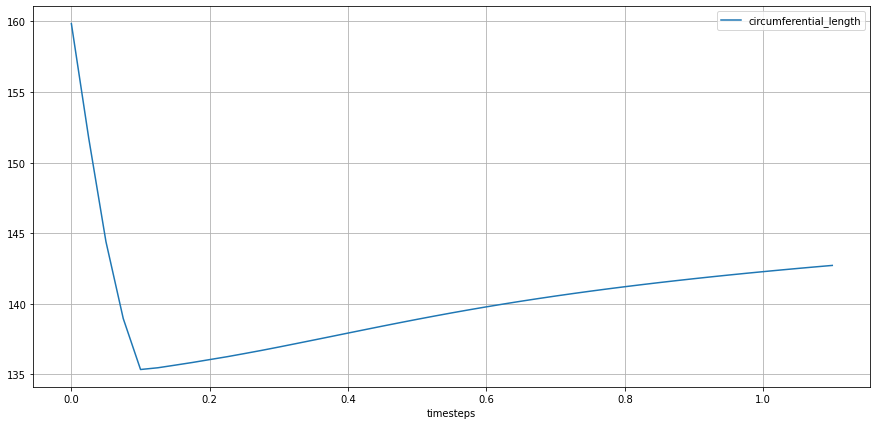
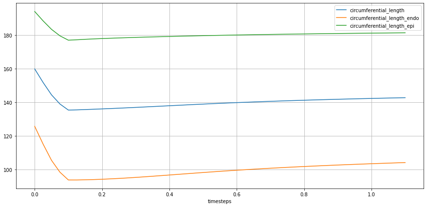
Similarly to ‘longitudinal length, the final computation of ’circumferential length’ is the result of the reduction of the sum of the reduced values of individual groups formed by ‘group’ and ‘name’, which essentially composes the target line for the given geometric metric.
For instance, this is a sample group formed by speckles’ ‘group’ and ‘name’ values:
[6]:
sample_spk_ideal = lv_ideal.get_speckles(spk_name="SAMPLE", spk_group="epi", spk_collection="SAMPLE")
lv_ideal.plot_speckles(sample_spk_ideal,
cmap="tab20",
point_size=200,
add_k_centers=True,
k_centers_as_line=True,
k_bins=False,
t=0)
At the end, the final result is the reduction of the length of each of these groups:
[7]:
sample_spk_ideal = lv_ideal.get_speckles(spk_collection="circ-6")
lv_ideal.plot_speckles(sample_spk_ideal,
cmap="jet",
point_size=200,
add_k_centers=False,
k_centers_as_line=False,
k_bins=False,
t=0)
However, considering that these lines are not fully connected, distorsions might occur at points of discontinuities and the full length of the desired line might not be achieved (depending on number of clusters and mesh size). Therefore, to account for possible errors, we define the ‘global longitudinal length’ separately.
Nonetheless, the described approach can be used to compute local longitudinal lengths by reducing subset values.
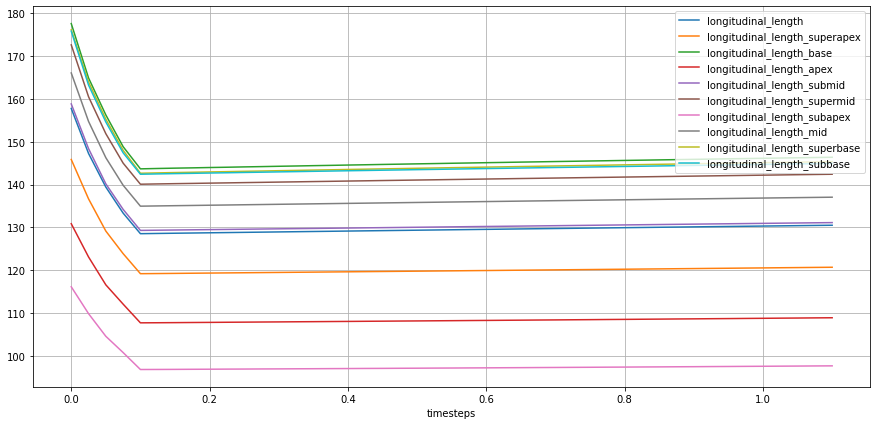
[8]:
long_spks = lv_ideal.get_speckles(spk_collection="circ-6")
lv_ideal.longitudinal_length(
long_spks,
approach="k_ids",
recompute=True,
reduce_by={"group", "name"},
log_level=logging.WARN,
)
lv_ideal.plot_metric(lv_ideal.STATES.LONG_LENGTH,
from_ts=0.0,
plot_infos={"group", "name"},
plot_infos_only=False,
# plot_infos_only_on_info_plots=True
)
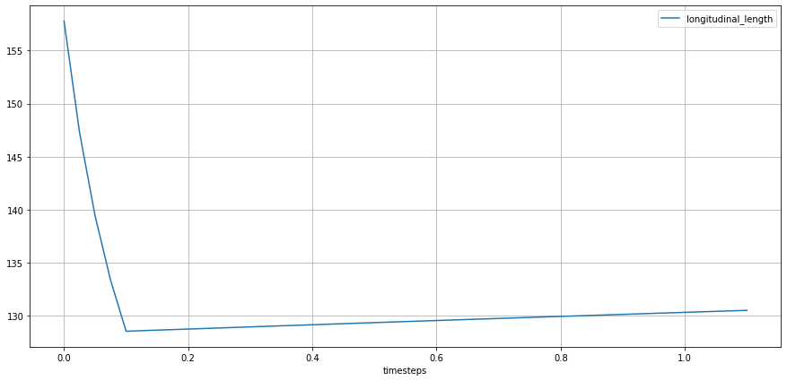
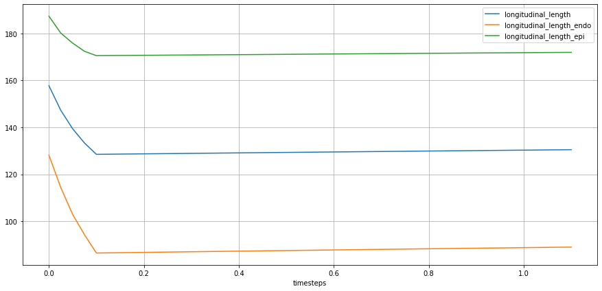
TODO:
add reduction by subset and group (will result in same similar graph but with individual values for endo-epi)
add option to save ‘circumferential length’ as the reduction of subsets, instead of sum (might be useful for detailed explanations)
Global circumferential length (TODO)#
As previously stated, discontinuities between cluster centers within speckle subsets might cause inaccuracies in calculating the total length of the required curve. While finer meshes and an increase in the number of clusters among speckles lessen this inaccuracy, we explored the notion of “global longitudinal speckle” as a separate technique for clarity and extended usage.
The global longitudinal length is defined as the length across the whole speckle and is meant for usage with speckles that do not contain subsets. In essence, we use the previously mentioned approach to compute length over a single speckle that covers the entire region of interest. The end effect is that all selected speckles are reduced while keeping consistency wihtin speckles (without discontinuities induced by subsets). Consider the following example:
TODO: fix visualization (join ends on circ lines)
[9]:
sample_spk_typeA = lv_ideal.get_speckles(spk_name="base", spk_group="epi", spk_collection="circ-1")
lv_ideal.plot_speckles(sample_spk_typeA,
cmap="hot",
point_size=200,
add_k_centers=True,
# k_centers_as_line=True,
k_bins=True,
# k_center_filters=dict(
# mfilter_ws=5,
# sfilter_ws=9,
# sfilter_or=1,
# keep_first=False,
# keep_last=False)
)
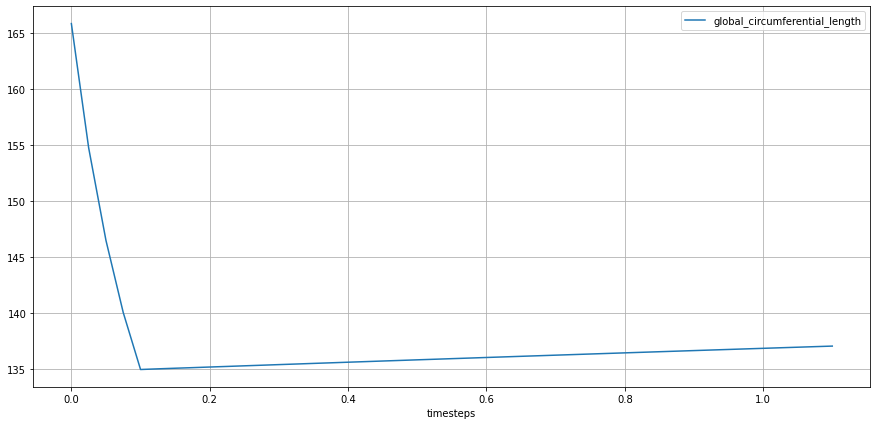
The final metric is shown below:
[10]:
long_spks = lv_ideal.get_speckles(spk_collection="circ-1")
lv_ideal.global_circumferential_length(
long_spks,
approach="k_ids",
recompute=True,
reduce_by={"group"},
log_level=logging.WARN,
# line_seg_filter_kwargs=dict(
# mfilter_ws=3,
# sfilter_ws=9,
# sfilter_or=1,
# keep_first=True,
# keep_last=True)
)
lv_ideal.plot_metric(lv_ideal.STATES.GLOBAL_CIRCUMFERENTIAL_LENGTH,
from_ts=0.0,
plot_infos=["group"])
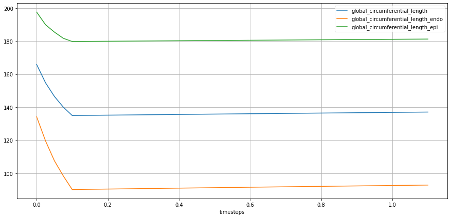
Although the computation of local speckles is helpful for detailed information about the myocardium, it is not often used in a clinical setting as values may vary from different vendors and different computation approaches. A recommended standard practice is to report values at Endocardium.